See ‘maximize_lp’ In Action

Linear Programming serves as a method for addressing real-world problems where the goal is to maximize (e.g., profit or security) or minimize (e.g., costs or risks) a certain outcome. Optimization is achieved by selecting appropriate values for variables, which are subject to various constraints. The mathematical model for such problems consists solely of linear expressions, excluding the multiplication of variables or raising them to a power. Many real-world optimization problems exhibit linear characteristics or can be linearized with minimal error.

For instance, consider the following example:

A company makes two types of cloth, X and Y, using three different colors of wool (see Fig 1). Cloth X yields a profit of $12 per unit, while cloth Y yields $8 per unit. The objective is to determine the optimal quantities of X and Y to maximize profit.

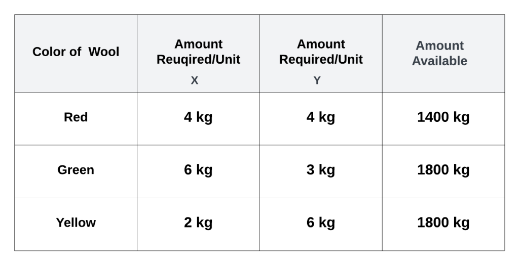
Fig. 1

Let and denotes the quantities of cloth X and Y produced, respectively. The profit is expressed as

Given that there is only kg of red wool available, and each cloth require kg of red wool, the constraint is

Similarly, considering the available green and yellow wool, the constraints are

Additionally, neither nor should be negative,

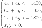
Therefore, the optimization problem can be formulated as:

Maximize the linear objective function

subject to the linear constraints:

The problem can be solved using Maxima’s ‘maximize_lp’ :

Fig. 2

The solution in Fig. 3 shows that the company should produce units of cloth X and units of cloth Y to achieve the maximum possible profit of $ This will utilize all the available red and green wool, leaving kg of yellow unused.

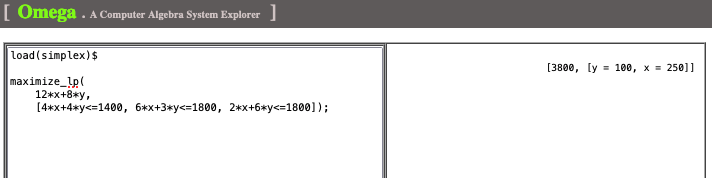
Fig. 3

See also “Building the Optimal Portfolio“

---