February 2020

In Memory of Dr. Li WenLiang (1986-2020)

This post is an introduction to deterministic models of infectious diseases and their Computer Algebra-Aided mathematical analysis.

We assume the followings for the simplistic SI model:

(A1-1) The population $N$ under consideration remains a constant.

(A1-2) The population is divided into two categories: the infectious and the susceptible. Their percentages are denoted by $i(t)$ and $s(t)$ respectively. At $t=0, i(0) = i_0$ .

(A1-3) The infectious’ unit time encounters with other individuals is $\lambda$ . Upon an encounter with the infectious, the susceptible becomes infected.

When a infectious host have $\lambda$ encounters with the population, $\lambda\cdot s(t)$ susceptible become infected. There are $N\cdot i(t)$ infectious in total at time $t$ . It means that within any time interval $[t, t+\Delta t]$ , the infectious will increase by $N\cdot i(t) \cdot \lambda s(t)\cdot \Delta t$ . i.e.,

$N\cdot i(t+\Delta t) -N\cdot i(t) = N\cdot i(t)\cdot\lambda s(t)\cdot\Delta t$ .

Cancelling out the $N$ ‘s,

$\frac{i(t+\Delta t)-i(t)}{\Delta t} = \lambda\cdot i(t) s(t)$

and so

$\lim\limits_{\Delta t\rightarrow 0}\frac{i(t+\Delta t)-i(t)}{\Delta t} = \lambda i(t) s(t)$ .

That is,

$\frac{d i(t)}{dt} = \lambda\cdot i(t) s(t)$ .

Deduce further from (A1-2) ( $i+s=1$ ) is that

$\begin{cases} \frac{d i}{dt} = \lambda i (1-i) \\ i(0) = i_0 \end{cases}\quad\quad\quad(1-1)$

Let’s examine (1-1) qualitatively first.

We see that the SI model has two critical points:

$i_1^* = 0, \quad i_2^* = 1$ .

$\forall i \in (0, 1), \frac{d i}{dt} = i(1-i) > 0 \implies \lim\limits_{t \rightarrow \infty} i(t)=1$ .

This indicates that in the presence of any initial infectious hosts, the entire population will be infected in time. The rate of infection is at its peak when $i = 0.5$ .

The qualitative results can be verified quantitatively by Omega CAS Explorer.

Fig. 1-1

From Fig. 1-1, we see that

$i(t) = \frac{1}{1-(1-\frac{1}{i_0})e^{-\lambda t}}$ .

Therefore,

$\lim\limits_{t \rightarrow \infty} i(t) = \lim\limits_{t \rightarrow \infty} \frac{1}{1-(1-\frac{1}{i_0})e^{-\lambda t}} = 1$ .

Fig. 1-2 confirms that the higher the number of initial infectious hosts( $i_0$ ), the sooner the entire population becomes infected ( $i = 1$ )

Fig. 1-2

The SI model does not take into consideration any medical practice in combating the spread of infectious disease. It is pessimistic and unrealistic.

An improved model is the SIR model. The assumptions are

(A2-1) See (A1-1)

(A2-2) See (A1-2)

(A2-3) See (A1-3)

and,

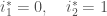
(A2-4) Number of individuals recovered from the disease in unit time is $\mu$ . The recovered are without immunity. They can be infected again.

By (A2-1) – (A2-4), the modified model is

$N \frac{d i}{dt} = \lambda N s i - \mu N i$

or,

$\begin{cases} \frac{d i}{dt} = \lambda i \cdot(1-i)-\mu\cdot i \\ i(0) = i_0 \end{cases}$

Let

$\sigma = \frac{\lambda}{\mu}$ ,

we have

$\begin{cases} \frac{d i}{dt} = -\lambda i \cdot(i - (1-\frac{1}{\sigma}))\\ i(0) = i_0 \end{cases}\quad\quad\quad(2-1)$

The new model has two critical points:

$i_1^*=0, \quad i_2^* = 1-\frac{1}{\sigma}$ .

And,

$\frac{d^2i}{dt^2} =\frac{d}{dt}(\frac{di}{dt})=\frac{d}{di}(-\lambda i (i-(1-\frac{1}{\sigma})))\cdot \frac{di}{dt}=-2\lambda (i-\frac{1}{2}(1-\frac{1}{\sigma}))\cdot \frac{di}{dt}$

i.e.,

$\frac{d^2i}{dt^2} = 2\lambda^2 i\cdot (i-\frac{1}{2}(1-\frac{1}{\sigma}))\cdot (i-(1-\frac{1}{\sigma}))$

Without solving (2-1), we extract from it the following qualitative behavior:

Case-1 $\sigma > 1$

[2-1-1] $\lim\limits_{t \rightarrow \infty} i(t) = 1-\frac{1}{\sigma}$

[2-1-2] $\forall i>1-\frac{1}{\sigma}, \frac{di}{dt} < 0$ .

[2-1-3] $\forall i < 1-\frac{1}{\sigma}, \frac{di}{dt} > 0$ .

[2-1-4] $i > 1-\frac{1}{\sigma}, \frac{d^2i}{dt^2} > 0$ .

[2-1-5] $\forall (\frac{1}{2}(1-\frac{1}{\sigma}) < i < (1-\frac{1}{\sigma})), \frac{d^2i}{dt^2} < 0$ .

[2-1-6] $\forall(0 < i < \frac{1}{2}(1-\frac{1}{\sigma})), \frac{d^2i}{dt^2} > 0$ .

Case-2 $\sigma < 1$

[2-2-1] $\lim\limits_{t\rightarrow \infty} i(t) = 0$ .

[2-2-2] $\forall i, \frac{di}{dt} < 0$ .

[2-2-3] $\forall i, \frac{d^2i}{dt^2} >0$ .

Case-3 $\sigma = 1$

[2-3-1] $\lim\limits_{t\rightarrow \infty} i(t) = 0$ .

[2-3-2] $\forall i, \frac{di}{dt} < 0$ .

[2-3-3] $\forall i, \frac{d^2i}{dt^2} >0$ .

The cases are illustrated by solving (2-1) analytically using Omega CAS Explorer (see Fig. 2-1,2-2,2-3)

Fig. 2-1 $\sigma> 1, i$ approaches $1-\frac{1}{\sigma}$ asymptotically.

Fig. 2-2 $\sigma < 1, i$ approaches $0$ asymptotically.

Fig. 2-3 $\sigma = 1, i$ approaches $0$ asymptotically.

Fig. 2-4 $\sigma > 1, i$ ‘s monotonicity depends on $i_0$ .

Fig. 2-4 shows that for $\sigma > 1$ , if $\frac{1}{2}(1-\frac{1}{\sigma})< i_0 < 1-\frac{1}{\sigma}$ , then $i$ increases on a convex curve. Otherwise, $\forall i_0 < \frac{1}{2}(1-\frac{1}{\sigma}), i$ increases on a concave curve first. The curve turns convex after $i$ reaches $\frac{1}{2}(1-\frac{1}{\sigma})$ . However, $\forall i_0 > (1-\frac{1}{\sigma}), i$ monotonically decreases along a concave curve.

Fig. 2-5 $\sigma < 1, i$ monotonically decrease.

Fig 2-5 illustrates the case $\sigma >1$ .

We also have:

Fig. 2-6 $\sigma =1, i$ monotonically decrease.

From these results we may draw the following conclusion:

If $\sigma >1$ , the monotonicity of $i(t)$ depends on the level of $i_0$ . Otherwise ( $\sigma = \frac{\lambda}{\mu} \le 1$ ), $i(t)$ will decrease and approach to $0$ since the rate of recovery from medical treatment $\mu$ is at least on par with the rate of infection $\lambda.$

This model is only valid for modeling infectious disease with no immunity such as common cold, dysentery. Those who recovered from such disease become the susceptible and can be infected again.

However, for many disease such as smallpox, measles, the recovered is immunized and therefore, falls in a category that is neither infectious nor susceptible. To model this type of disease, a new mathematical model is needed.

Enter the Kermack-McKendrick model of infectious disease with immunity.

There are three assumptions:

(A3-1) The total population $N$ does not change.

(A3-2) Let $i(t), s(t)$ and $r(t)$ denote the percentage of the infectious, susceptible and recovered respectively. At $t=0, i(0) = i_0, s(0) = s_0, r(0) = r_0 = 0$ . The recovered are the individuals who have been infected and then recovered from the disease. They will not be infected again or transmit the infection to others.

(A3-3) $\lambda$ is the unit time number of encounters with the infectious, $\mu$ the unit time recoveries from the disease.

For the recovered, we have

$N\frac{dr}{dt} = \mu N i$ .

Hence,

$\begin{cases} \frac{d i(t)}{dt} = \lambda s(t) i(t) - \mu i(t),\;i(0) = i_0\quad\quad\; (3-1-1)\\ \frac{d s(t)}{dt} = -\lambda s(t)i(t),\;s(0) = s_0\quad\quad\quad\quad\;\;(3-1-2) \\ \frac{d r(t)}{dt} = \mu i(t),\;r(0)=r_0=0\quad\quad\quad\quad\;\;\;\;(3-1-3)\\i_0, s_0 \in (1, 0), i_0+s_0=1\quad\quad\quad\quad\quad\;\;\;\;(3-1-4)\end{cases}$

This system of differential equations appears to defy any attempts to obtain an analytic solution (i.e., no solution can be expressed in terms of known function).

Numerical treatments for two sets of given $\lambda, \mu$ and $(s_0, i_0)$ are depicted in Fig. 3-1 and Fig. 3-2.

Fig. 3-1 $\lambda = 0.25, \mu=0.1, i_0= 0.15, s_0=0.85$

Fig. 3-2 $\lambda = 0.25, \mu=0.1, i_0=0.75, s_0=0.25$

However, it is only the rigorous analysis in general terms gives the correct interpretations and insights into the model.

To this end, we let

$\rho = \frac{\mu}{\lambda}$ .

For $\frac{ds}{dt} \ne 0 (i.e., i \ne 0, s \ne 0)$ ,

$\frac{\frac{di}{dt}}{\frac{ds}{dt}} = \frac{di}{ds} = -1+\rho\frac{1}{s}$

or,

$\frac{di}{ds} = -1+\rho\frac{1}{s}.$

It has the following qualitatives:

[3-1] $\forall s < \rho, \frac{di}{ds} > 0 \implies i$ increases.

[3-2] $s = \rho, \frac{di}{ds} = 0\implies i$ reaches its maximum.

[3-3] $\forall s>\rho, \frac{di}{ds} < 0\implies i$ decreases.

The analytical solution to

$\begin{cases} \frac{di}{ds} = -1+\frac{\rho}{s}\\ i(s_0) = i_0\end{cases}\quad\quad\quad(3-2)$

(see Fig. 3-3) is

$i(s) = \rho\log(\frac{s}{s_0}) -s +i_0+s_0 \overset{[3-1-4]}{=} \rho\log(\frac{s}{s_0}) -s +1\quad\quad\quad(3-3)$

Fig. 3-3

Notice that

$\forall s, (s, 0)$ is a critical point of (3-1-1) and (3-1-2).

or,

all points on the s-axis of the s-i phase plane are critical points of (3-1-1) and (3-1-2).

By a theorem of qualitative theory of ordinary differential equations (see Fred Brauer and John Nohel: The Qualitative Theory of Ordinary Differential Equations, p. 192, Lemma 5.2),

$\forall t>0, i(t)>0\quad\quad\quad(3-4)$

Moreover, let $s' = s_0e^{-\frac{1}{\rho}},$

$i(s')=1-s' + \rho\log(\frac{s'}{s_0}) <1 + \rho\log(\frac{s'}{s_0}) = 1+ \rho\log(\frac{s_0e^{-\frac{1}{\rho}}}{s_0})=1+\rho\cdot(-\frac{1}{\rho})=0$

i.e.,

$i(s') < 0\quad\quad\quad(3-5)$

Since $s' = s_0e^{-\frac{1}{\rho}} = \frac{s_0}{e^{\frac{1}{\rho}}} \overset{\frac{1}{\rho}>0\implies e^{\frac{1}{\rho}}>e^0=1}{<} s_0$ , together, (3-5) and $i(s_0) = i_0 >0$ implies

$\exists s_{\infty} : s' < s_{\infty}<s_0 \ni 1-s_{\infty} + \rho \log(\frac{s_{\infty}}{s_0})=0$

or,

$\exists s_{\infty} : 0 \overset{s' = s_0e^{-\frac{1}{\rho}}> 0}{<} s_{\infty} < s_0 \ni 1-s_{\infty} + \rho\log(\frac{s_{\infty}}{s_0})=0.$

Clearly, $(s_{\infty}, 0)$ is a critical point of (3-1-1) and (3-1-2). Lemma 5.2 thus ensures

$\forall t>0, s(t) > s_{\infty} > 0\quad\quad\quad(3-6)$

It follows that

$\forall t>0, \frac{ds(t)}{dt} = -\lambda i(t)\cdot s(t) \overset{(3-4), (3-6)}{<} 0\quad\quad\quad(3-7)$

To the list ([3-1]-[3-3]) , we now add:

[3-4] $\forall t_2> t_1>0, s(t_2) \overset{(3-7)}{<} s(t_1)$

[3-5] $\lim\limits_{t \rightarrow \infty} i(t) = 0, \lim\limits_{t \rightarrow \infty} s(t) = s_{\infty}$

[3-6] $\forall t>0, \frac{dr(t)}{dt} = \mu i(t) \overset{(3-4)}{>}0$

And so, for all $(s_0, i_0) : 0 < s_0 <1, 0<i_0 < 1$ ,

if $\rho < s_0 <1$ then

$\forall s_+: \rho \le s_+ < s_0, i_+ = i(s_+) \overset{[3-1], [3-4], (3-1-4)}{>} i(s_0)=i_0.$

Since

$i_{max} \overset{[3-2]}{=} i(\rho) \overset{(3-3)}{=} \rho\log(\frac{\rho}{s_0})-\rho+1\overset{s_0 > \rho \implies \frac{\rho}{s_0} < 1 \implies \log(\frac{\rho}{s_0}) < 0}{<}1\quad\quad\quad(3-8),$

we have

$\forall s_+: 0 < s_+ \le \rho, i_+ = i(s_+) \le i_{max} < 1.$

Fig. 3-4

If $s_0=\rho$ then,

$i_+ = i(s_+ < \rho) \overset{[3-2], [3-4]}{<} i_{max} \overset{(3-8)}{<} 1.$

Fig. 3-5

If $0 <s_0 < \rho$ then

$i_+=i(s_+ < s_0) \overset{[3-1], [3-4]}{<} i(s_0)=i_0 < 1.$

Fig. 3-6

In fact, for all finite $t>0$ ,

$\forall s_+ : 0<s_+ <s_0, i_+ = i(s_+) <1$ .

Thus, the orbits of (3-1-1) and (3-1-2) have the form illustrated in Fig. 3-7.

Fig. 3-7

For example,

Fig. 3-8 $\rho=0.3$

What we see is that as time $t$ advances, $(i(t), s(t))$ moves along the curve (3-3) in the direction of decreasing $s.$ Consequently, if $s_0$ is less than $\rho$ , then $i(t)$ decreases monotonically to $0$ , and $s(t)$ decreases to $s_{\infty}$ . Therefore, if a small group of infectious $i_0$ is introduced into the population with the susceptibles $s_0$ , with $s_0 < \rho$ , the disease will die out rapidly. On the other hand, if $s_0$ is greater than $\rho$ , then $i(t)$ increases as $s(t)$ decreases to $\rho$ . Only after attaining its maximum at $s=\rho, i(t)$ starts to decrease when the number of susceptibles falls below the threshold value $\rho.$

We therefore conclude:

An epidemic will occur only if the number of susceptibles in a population exceeds the threshold value $\rho$ .

It means a larger $\rho$ is preferred.

To increase $\rho = \frac{\mu}{\lambda}$ , the recovery rate $\mu$ is boosted through adequate medical care and treatment. Meanwhile, $\lambda$ is reduced by quarantine and social distancing.

In addition to increase $\rho$ , we can also decrease $s_0$ through immunizing the population.

If the number of susceptibles $s_0$ is initially greater than, but close to the threshold value $\rho$ :

$\rho < s_0 \approx \rho\quad\quad\quad(3-9)$ ,

and $i_0$ is very small compared to $s_0$ :

$i_0 \ll s_0\quad\quad\quad(3-10)$ ,

we can estimate the number of individuals who ultimately contracted the disease.

From (3-1-4), we have

$s_0+i_0+0=1\quad\quad\quad(3-11)$

and $\lim\limits_{t\rightarrow \infty}(s(t) + i(t) + r(t))$ yields

$s_{\infty} + 0 + r_{\infty} = 1\quad\quad\quad(3-12)$

(3-11)-(3-12),

$s_0-s_{\infty} + i_0 - r_{\infty} =0 \overset {(3-10)}{\implies} s_0 - s_{\infty} - r_{\infty} = 0$

or,

$r_{\infty} = s_0 - s_{\infty}\quad\quad\quad(3-13)$

Given (3-9), we deduce from it that

$1< \frac{s_0}{\rho} \approx 1 \implies 0 < \frac{s_0}{\rho}-1 \approx 0 \implies 0 <\frac{s_0-\rho}{\rho} \approx 0\implies 0 <\frac{s_0-\rho}{\rho} \ll 1$

i.e.,

$\rho < s_0 \approx \rho \implies 0<\frac{s_0-\rho}{\rho} \ll 1\quad\quad\quad(3-14)$

(3-1-2) / (3-1-3) gives

$\frac{\frac{ds}{dt}}{\frac{dr}{dt}}=\frac{ds}{dr} = -\frac{\lambda}{\mu}s=-\frac{1}{\rho}s$

Solving

$\begin{cases} \frac{ds}{dr} =-\frac{1}{\rho}s\\s(r_0=0)=s_0\end{cases}$

yields

$s = s_0 e^{-\frac{r}{\rho}}\quad\quad\quad(3-15)$

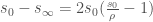
After substituting (3-15) in (3-1-3),

$\frac{dr}{dt} = \mu(1-r-s) \overset{(3-14)}{=}\mu(1 - r -s_0 e^{-\frac{r}{\rho}})\quad\quad\quad(3-16)$

In view of the fact that

$\frac{r}{\rho} \overset{[3-6]}{<} \frac{s_0-s_{\infty}}{\rho} \overset{(3-9)}{\approx} \frac{s_0-s_{\infty}}{s_0}<1\quad\quad\quad(3-17)$ ,

we approximate the term $e^{-\frac{r}{\rho}}$ in (3-16) with a Taylor expression up to the second order (see Fig. 3-9)

Fig. 3-9

The result is an approximation of equation (3-16):

$\frac{dr}{dt}=\mu(1-r-s_0(1-\frac{r}{\rho}+\frac{r^2}{2\rho^2}))$

i.e.,

$\frac{dr}{dt}=\mu(1-s_0+(\frac{s_0}{\rho}-1)r-\frac{s_0}{2\rho^2}r^2)$

It can be solved analytically (see Fig. 3-10).

Fig. 3-10

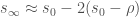
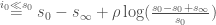
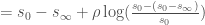
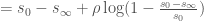
As a result,

$\lim\limits_{t \rightarrow \infty} r(t) = 2\rho(1-\frac{\rho}{s_0})\quad\quad\quad(3-18)$

It follows from

$2\rho(1-\frac{\rho}{s_0}) = 2\rho (\frac{s_0-\rho}{s_0}) =2(s_0-\rho)(\frac{\rho}{s_0-\rho+\rho})=2(s_0-\rho)(\frac{1}{1+\frac{s_0-\rho}{\rho}}) \overset{(3-13)}{\approx} 2(s_0-\rho)$

that (3-18) yields

$r_{\infty} \approx 2(s_0-\rho)$

Namely, the size of the epidemic is roughly $2(s_0-\rho)$ . Consequently, by (3-13),

$s_{\infty} = s_0 - 2(s_0-\rho)$ .

The above analysis leads to the following threshold theorem of epidemiology:

(a) An epidemic occurs if and only if $s_0$ exceeds the threshold $\rho$ .

(b) If $\rho<s_0 \approx \rho$ and $i_0 \ll s_0$ , then after the epidemic, the number of susceptible individuals is reduced by an amount approximately $2(s_0-\rho)$ , namely, $s_{\infty} \approx s_0-2(s_0-\rho)$ .

We can also obtain (b) without solving for $r(t)$ :

From (3-3), as $t\rightarrow \infty$ ,

$0 =\rho \log(\frac{s_{\infty}}{s_0})-s_{\infty} + i_0 + s_0$

$\overset{i_0 \ll s_0}{=} s_0 - s_{\infty} + \rho\log(\frac{s_0-s_0+s_{\infty}}{s_0})$

$= s_0 -s_{\infty} + \rho\log(\frac{s_0-(s_0-s_{\infty})}{s_0})$

$= s_0 -s_{\infty} + \rho\log(1-\frac{s_0-s_{\infty}}{s_0})$

When $s_0-s_{\infty}$ is small compared to $s_0$ (see (3-17)), we approximate $\log(1-\frac{s_0-s_{\infty}}{s_0})$ with a truncated Taylor series after two terms. Namely,