Snowflake and Anti-Snowflake Curves

July 27, 2020July 30, 2020 / Michael Xue / Leave a comment

Fig. 1

The snowflake curve made its first appearence in a 1906 paper written by the Swedish mathematician Helge von Koch. It is a closed curve of infinite perimeter that encloses a finite area.

Start with a equallateral triangle of side length $a$ and area $A_0$ , the snowflake curve is constructed iteratively (see Fig. 1). At each iteration, an outward equallateral triangle is created in the middle third of each side. The base of the newly created triangle is removed:

Fig. 2

Let $s_i$ be the number of sides the snowflak curve has at the end of $i^{th}$ iteration. From Fig. 2, we see that

$\begin{cases}s_i = 4s_{i-1}\\ s_0=3\end{cases}$ .

Fig. 3

Solving for $s_i$ (see Fig. 3) gives

$s_i = 3\cdot 4^i.$

Suppose at the end of $i^{th}$ iteration, the length of each side is $a^*_i$ , we have

$\begin{cases}a^*_i = \frac{a^*_{i-1}}{3}\\ a^*_0=a\end{cases}$ ,

therefore,

$a^*_i = (\frac{1}{3})^i a$

and, $p_i$ , the perimeter of the snowflake curve at the end of $i^{th}$ iteration is

$p_i = s_{i-1} (4\cdot a^*_i) = (3\cdot4^{i-1})\cdot (4\cdot(\frac{1}{3})^ia)=3(\frac{4}{3})^i a$ .

It follows that

$\lim\limits_{i\rightarrow \infty}p_i =\infty$

since $|\frac{4}{3}|>1$ .

Let $A^*_{i-1}, A^*_i$ be the area of equallateral triangle created at the end of $(i-1)^{th}$ and $i^{th}$ iteration respectively. Namely,

$A^*_{i-1} = \boxed{\frac{1}{2}a^*_{i-1}\sqrt{(a^*_{i-1})^2-(\frac{a^*_{i-1}}{2})^2}}$

and

$A^*_{i} = \frac{1}{2}\frac{a^*_{i-1}}{3}\sqrt{(\frac{a^*_{i-1}}{3})^2-(\frac{1}{2}\frac{a^*_{i-1}}{3})^2}= \frac{1}{9}\cdot\boxed{\frac{1}{2}a^*_{i-1}\sqrt{(a^*_{i-1})^2-(\frac{a^*_{i-1}}{2})^2}}=\frac{1}{9}A^*_{i-1}$ .

Since

$\begin{cases}A^*_i = \frac{1}{9} A^*_{i-1} \\ A^*_0=A_0\end{cases}$ ,

solving for $A^*_i$ gives

$A^*_i = (\frac{1}{9})^i A_0$ .

Hence, the area added at the end of $i^{th}$ iteration

$\Delta A_i = s_{i-1} A^*_i = (3\cdot4^{i-1})\cdot(\frac{1}{9})^{i}A_0$ .

After $n$ iterations, the total enclosed area

$A_n =A_0 + \sum\limits_{i=1}^{n}\Delta A_i = A_0 + \sum\limits_{i=1}^{n}(3\cdot4^{i-1})\cdot(\frac{1}{9})^i A_0=\frac{8}{5}A_0-\frac{3}{5}(\frac{4}{9})^{n}A_0$ .

As the number of iterations tends to infinity,

$\lim\limits_{n\rightarrow \infty}A_n = \frac{8}{5}A_0$ .

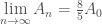
i.e., the area of the snowflake is $\frac{8}{5}$ of the area of the original triangle.

If at each iteration, the new triangles are pointed inward, the anti-snowflake is generated (see Fig. 4 ).

Fig. 4 First four iterations of anti-snowflake curve

Like the Snowflake curve, the perimeter of the anti-snowflake curve grows boundlessly, whereas its total enclosed area approaches a finite limit (see Exercise-1).

Exercise-1 Let $A_0$ be the area of the original triangle. Show that the area encloded by the anti-snowflake curve approaches $\frac{5}{2}A_0$ .

Exercise-2 An “anti-square curve” may be generated in a manner similar to that of the anti-snowflake curve (see Fig. 5). Find:

(1) The perimeter at the end of $i^{th}$ iteration

(2) The enclosed area at the end of $i^{th}$ iteration

Fig. 5 First four iterations of anti-square curve

An Edisonian Moment

July 14, 2020September 27, 2022 / Michael Xue / Leave a comment

We are told that shortly after Edison invented the light bulb, he handed the glass section of a light bulb to one of his engineers, asking him to find the volume of the inside. This was quite a challenge to the engineer, because a light bulb is such an irregular shape. Figuring the volume of the bulb’s irregular shape was quite different from figuring the volume of a glass, or a cylinder.

Several days later, Edison passed the engineer’s desk, and asked for the volume of the bulb, but the engineer didn’t have it. He had been trying to figure the volume mathematically, and had some problems because the shape was so irregular.

Edison took the bulb from the man; filled the bulb with water; poured the water into a beaker, which measured the volume, and handed it to the amazed engineer.

Vincent A. Miller, Working with Words, Words to Work With, 2001, pp. 57-58

“Analyze This!” shows the equilibrium point $(x_*, y_*)$ of

$\begin{cases}\frac{dx}{dt}=n k_2 y - n k_1 x^n\\ \frac{dy}{dt}=k_1 x^n-k_2 y\\x(0)=x_0, y(0)=y_0\;\end{cases}$

can be found by solving equation

$-nk_1x^n-k_2x+c_0=0$

where $k_1>0, k_2>0, c_0>0$ .

When $n=4$ , Omega CAS Explorer‘s equation solver yields a list of $x$ ‘s (see Fig. 1).

Fig. 1

It appears that identifying $x_*$ from this list of formidable looking expressions is tedious at best and close to impossible at worst:

Fig. 2

However, by Descartes’ rule of signs ,

$\forall k_1>0, k_2>0, c_0>0, -4k_1x^4-k_2x+c_0=0$ has exactly one positive root.

It means that $x_*$ can be seen quickly from evaluating the $x$ ‘s numerically with arbitrary chosen positive values of $k_1, k_2$ and $c_0$ . For instance, $k_1=1, k_2=1, c_0=1$ (see Fig. 3).

Fig. 3

Only the second value is positive:

Therefore, $x_*$ is the second on the list in Fig. 1:

It’s Magic Square!

July 7, 2020October 6, 2022 / Michael Xue / Leave a comment

A magic square is a $n$ by $n$ square grid filled with distinct integers $1,2,..., n^2$ such that each cell contains a different integer and the sum of the integers, called magic number, is equal in each row, column and diagonal. The order of a $n$ by $n$ magic square is $n$ .

The first known example of a magic square is said to have been found on the back of a turtle by Chinese Emperor Yu in 2200 B.C. (see Fig. 1) : circular dots represents the integers 1 through 9 are arranged in a $3$ by $3$ grid. Its order and magic number are $3$ and $15$ respectively.

Fig. 1

The first magic square to appear in the Western world was the one depicted in a copperplate engraving by the German artist-mathematician Albrecht Dürer, who also managed to enter the year of engraving – $1514$ – in the two middle cells of the bottom row (see Fig. 2)

Fig. 2

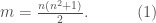
Let $m$ be the magic number of a $n$ by $n$ magic square. Sum of all its rows (see “Little Bird and a Recursive Generator“)

$n\cdot m = 1+2+3+...+n^2 = \frac{n^2(n^2+1)}{2}$ .

That is,

$m = \frac{n(n^2+1)}{2}.\quad\quad\quad(1)$

Fig. 3

There is no $2$ by $2$ magic square. For if there is, it must be true (see Fig. 3) that

$a +b = a+c \implies b=c$ , contradicts “each cell contains a different integer”.

Shown in Fig. 4 is a square whose rows and columns add up to $260$ , but the diagonals do not, which makes the square only semi-magic.

Fig. 4

What’s interesting is that a chess Knight, starting its L-shaped moves from the cell marked “ $1$ ” can tour all $64$ squares in numerical order. The knight can reach the starting point from its finishing cell (marked” $64$ “) for a new round of tour.

Exercise-1 Is it true that for every $n \in \mathbb{N}\setminus\left\{2\right\}$ there exists at least one magic square?

Exercise-2 Is there a Knight’s Tour magic square?

Exercise-3 Fill in the missing numbers in the following square so that it is a magic square: