Fig. 1
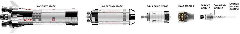
A rocket with stages is a composition of single stage rocket (see Fig. 1) Each stage has its own casing, instruments and fuel. The th stage houses the payload.
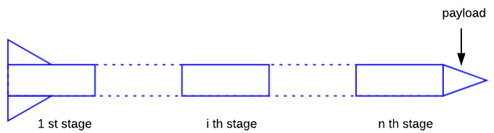
Fig. 2
The model is illustrated in Fig. 2, the stage having initial total mass
  and containing fuel
  . The exhaust speed of the stage is
  .
The flight of multi-stage rocket starts with the
.
The flight of multi-stage rocket starts with the  stage fires its engine and the rocket is lifted. When all the fuel in the stage has been burnt, the stage’s casing and instruments are detached. The remaining stages of the rocket continue the flight with
  stage’s engine ignited.
Generally, the rocket starts its stage of flight with final velocity achieved at the end of previous stage of flight. The entire rocket is propelled by the fuel in the casing of the rocket. When all the fuel for this stage has been burnt, the casing is separated from the rest of the stages. The flight of the rocket is completed if
stage’s engine ignited.
Generally, the rocket starts its stage of flight with final velocity achieved at the end of previous stage of flight. The entire rocket is propelled by the fuel in the casing of the rocket. When all the fuel for this stage has been burnt, the casing is separated from the rest of the stages. The flight of the rocket is completed if  . Otherwise, it enters the next stage of flight.
When all external forces are omitted, the governing equation of rocket’s stage flight (see “Viva Rocketry! Part 1” or “An alternate derivation of ideal rocket’s flight equation“) is
. Otherwise, it enters the next stage of flight.
When all external forces are omitted, the governing equation of rocket’s stage flight (see “Viva Rocketry! Part 1” or “An alternate derivation of ideal rocket’s flight equation“) is

 to
to  ,
,

 when stage’s fuel has been burnt, we have


 the velocity of rocket at the end of
  stage of flight.
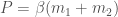
Since
stage of flight.
Since  , (2) becomes

i.e.,

For a single stage rocket (
 ), (3) is

In my previous post “Viva Rocketry! Part 1“, it shows that given 


 that will enable the single stage rocket to produce the speed a satellite needs?
Let’s find out.
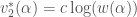
Differentiate (4) with respect to gives
that will enable the single stage rocket to produce the speed a satellite needs?
Let’s find out.
Differentiate (4) with respect to gives
 are positive quantities and
  .
It means
.
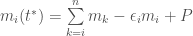
It means  is a monotonically decreasing function of .
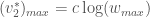
Moreover,
is a monotonically decreasing function of .
Moreover,
 , (5) yields approximately

Fig. 3
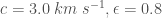
This upper limit implies that for the given and
and  , no value of will produce a speed beyond (see Fig. 4)
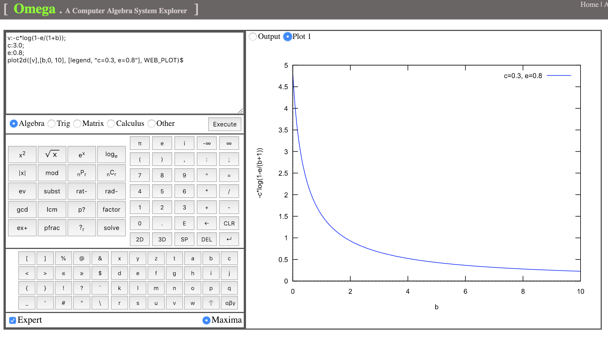
Fig. 4
Let’s now turn to a two stage rocket (
 )
From (3), we have
)
From (3), we have

 and
and  , then


 and
and  ,
,
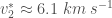
Fig. 5
This is a considerable improvement over the single stage rocket ( ). Nevertheless, it is still short of producing the orbiting speed a satellite needs.
In fact,
). Nevertheless, it is still short of producing the orbiting speed a satellite needs.
In fact,

 is a monotonically decreasing function of .
In addition,
is a monotonically decreasing function of .
In addition,

, the limit is approximately

Fig. 6
In the value used above, we have taken equal stage masses, . i.e., the ratio of
  .
Is there a better choice for the ratio of
.
Is there a better choice for the ratio of  such that a better can be obtained?
To answer this question, let
such that a better can be obtained?
To answer this question, let  , we have

 , by (8),


 a function of
  . It can be written as

 and
and  .
Since is a monotonic increasing function (see “Introducing Lady L“),
.
Since is a monotonic increasing function (see “Introducing Lady L“),
 denote the maximum of and respectively.
To find
denote the maximum of and respectively.
To find  , we differentiate ,

 for gives
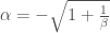

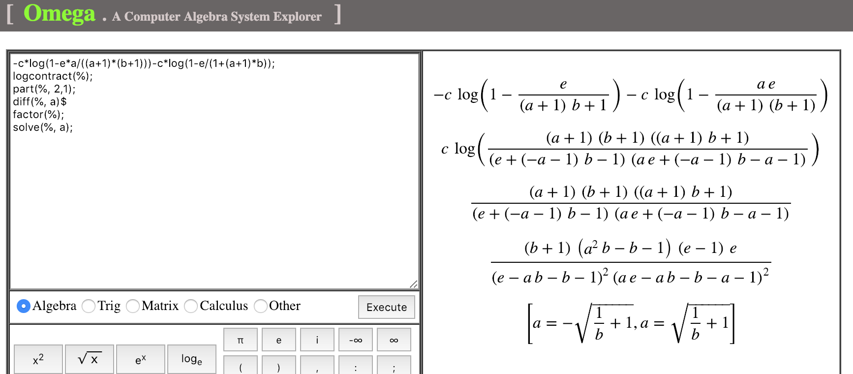
Fig. 7
By (8), the valid solution is
attains an extreme value at .
Moreover, we observe from (11) that

attains maximum at  .
It follows that
.
It follows that

 , the optimum ratio
  , showing that the first stage must be about ten times large than the second.
Using this ratio and keep
, showing that the first stage must be about ten times large than the second.
Using this ratio and keep  as before, (10) now gives

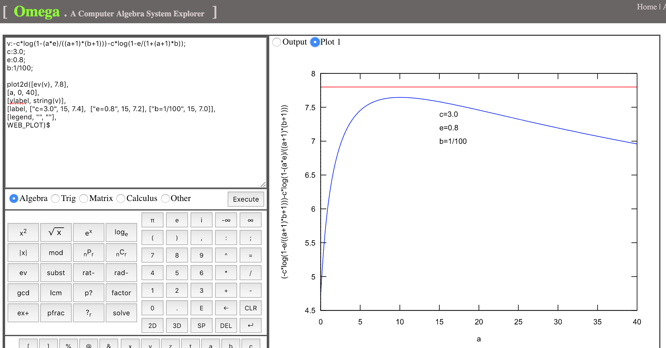
Fig. 8
Setting , we reach the goal:
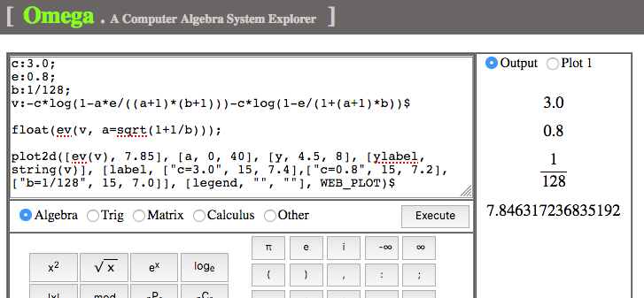
Fig. 9
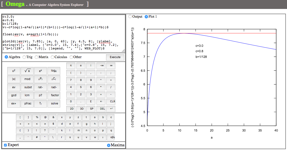
Fig. 10
At last, it is shown mathematically that provided the stage mass ratios ( and
and  )are suitably chosen, a two stage rocket can indeed launch satellites into earth orbit.
Exercise 1. Show that
 and .
Exercise 2. Using the optimum and , solving (10) numerically for such that
and .
Exercise 2. Using the optimum and , solving (10) numerically for such that  .
.
