Feuerbach’s Nine-Point Circle Theorem states that a circle passes through the following nine significant points of any triangle can be constructed:
1. The midpoint of each side of the triangle
2. The foot of each altitude
3. The midpoint of the line segment from each vertex of the triangle to the orthocenter
Let’s prove it with the aid of Omega CAS Explorer.

Step-1 Set up the circle equation:

is a circle centered at 
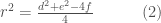
provide (2) is positive.
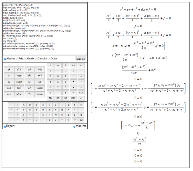
Step-2 Find d,e,f using p1, p2, p3:
ceq: x^2+y^2+d*x+e*y+f=0;
eq1: ev(ceq, x=(x1+x2)/2, y=y2/2);
eq2: ev(ceq, x=0, y=0);
eq3: ev(ceq, x=(x2-x1)/2, y=y2/2);
sol: linsolve([eq1, eq2, eq3], [d,e,f]);

The new circle equation is
nceq: ev(ceq, sol);

Evaluate (2)
ev(d^2+e^2-4*f, sol);

always positive for 
Step-3 Show p5, p6, p4 are on the circle:
p5:ev(nceq, x=x2, y=0);

p4: linsolve([(x2-x1)*y=y2*(x-x1), y2*y=-(x2-x1)*(x+x1)], [x,y]);
ratsimp(ev(nceq, p4));

p6: linsolve([(x2+x1)*y=y2*(x+x1), y*y2=-(x2+x1)*(x-x1)], [x,y]);
ratsimp(ev(nceq, p6));

Step-4 Find the orthocenter
o: linsolve([x=x2, y*y2=-(x2+x1)*(x-x1)], [x,y]);

Step-5 Show p7, p8, p9 are on the circle:
xo: rhs(o[1]);
yo: rhs(o[2]);
p7: ratsimp(ev(nceq, x=(xo+x2)/2, y=(yo+y2)/2));
p8: ratsimp(ev(nceq, x=(xo-x1)/2, y=(yo+0)/2));
p9: ratsimp(ev(nceq, x=(xo+x1)/2, y=(yo+0)/2));
This post is essentially my presentation at 21st Conference on Applications of Computer Algebra, July 20-23, 2015, Kalamata, Greece.

 and
and  , namely, we shall prove the following two propositions:

 ,
,
 when
when 
 both
both  are solutions of initial-value problem

 when
when 
 are solutions of initial-value problem
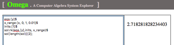
 . This constant is often denoted by
  and commonly known as Euler Number.
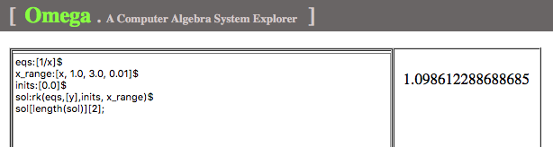
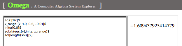
 from 1 to
  (see “
 is that the area under
  is 1 (see Fig. 1)
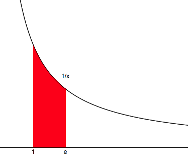
 where
where 
 where
where  ,
, and
and  are continuous positive functions.


 where
where  .
. where
where  .
.


 ,
,
 ,
, ,
,
 and
and  are solutions of initial-value problem
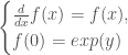
 .
.
 .
. then
then
 .
. .
. , i.e.,
  .
.
 ,
,

 and
and  are both solutions of initial-value problem
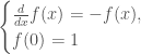
 .
.
 .
.
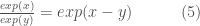
 . Using this notation, propositions (2), (3), (4), (5) are expressed as
 ,
, ,
, ,
,
 .”
.” .
.


 ,
,

 is a solution of the initial-value problem
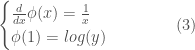

 ,
,
 is also a solution of (3)
 .
.
 :
:
 , when
  .
. .
.