Raindrops: Nature’s Serenade

August 19, 2023September 10, 2023 / Michael Xue / Leave a comment

A spherical falling raindrop leaves a cloud with initial radius $r_0$ and negligible speed. As it passes through the atmosphere, its mass increases at a rate proportional to the product of its surface area and speed $v.$ Assume its density is constant, show that its radius $r,$ increases linearly with $x,$ its distance below the cloud.

If $r_0$ is very small show that the acceleration of the raindrop is approximately $g-\frac{3v^2}{x}.$ Show also, when $r_0$ is very small, the equation that governs the motion of the raindrop can be written in the form

$\frac{dp}{dx} + \frac{6p}{x} = 2g,$

where $p=v^2.$ Verify that the equation has solution $p=\frac{2gx}{7}$ and show that the acceleration of the raindrop is $\frac{g}{7}.$

We know the mass of the spherical raindrop

$m = \rho\cdot\frac{4}{3}\pi r^3\quad\quad\quad(1)$

and, from “its mass increases at a rate proportional to the product of its surface area and speed”:

$\frac{dm}{dt} = k\cdot4\pi r^2\cdot v.\quad\quad\quad(2)$

Consequently,

$\frac{dm}{dt} \overset{(1)}{=} \rho\cdot 4\pi r^2 \frac{dr}{dt}\overset{(2)}{=}k\cdot4\pi r^2\cdot v\implies\frac{dr}{dt}\overset{\rho=1}{=}kv\implies \frac{dr}{dt}\overset{v=\frac{dx}{dt}}{=}k\frac{dx}{dt}.\quad\quad\quad(2)$

When $r_0$ is small ( $r_0 \approx 0$ ),

$r = kx, \quad\quad\quad(3)$

the raindrop’s radius increases linearly with $x,$ its distance below the cloud.

Applying Newton’s second law to the falling raindrop,

$\frac{d(mv)}{dt} = mg\quad\implies \quad \frac{dm}{dt}v + m\frac{dv}{dt} = mg.\quad\quad\quad(*)$

We find $\frac{dv}{dt}$ from $(*)$ as follows:

$m\frac{dv}{dt} = mg - \frac{dm}{dt}v,$

$\frac{dv}{dt} = g - \frac{1}{m}\frac{dm}{dt}v\overset{(1), (2)}{=} g - \frac{1}{\frac{4}{3}\pi r^3}k\cdot 4\pi r^2v\cdot v = g - \frac{3v^2k}{r}\overset{(3)}{=} g - \frac{3v^2k}{kx} = g - \frac{3v^2}{x}$

i.e.,

$\frac{dv}{dt} = g - \frac{3v^2}{x}.\quad\quad\quad(4)$

Now consider $\frac{m}{2}(\frac{dp}{dx} + \frac{6p}{x})$ where $p=v^2$ :

$\frac{m}{2}(\frac{\frac{dp}{dt}}{\frac{dx}{dt}} + \frac{6p}{x}) = \frac{m}{2}(\frac{2v\frac{dv}{dt}}{v} + \frac{6p}{x}) = m(\frac{dv}{dt} + \frac{3v^2}{x}) \overset{(4)}{=} m(g-\frac{3v^2}{x} + \frac{3v^2}{x}) = mg.$

That is,

$\frac{m}{2}(\frac{dp}{dx} + \frac{6p}{x}) = mg.\quad\quad\quad(5)$

Hence, (5) is an equivalent of $(*)$ . Its simplified form is:

$\frac{dp}{dx}+\frac{6p}{x} = 2g.$

Substituting $p=\frac{2gx}{7}$ into $\frac{dp}{dx}+\frac{6p}{x}$ gives

$\frac{2g}{7} +\frac{6}{x}\cdot \frac{2gx}{7} = \frac{2g}{7} + \frac{12g}{7} = \frac{14g}{7}=2g \implies p=\frac{2gx}{7}$ is a solution of $\frac{dp}{dx}+\frac{6p}{x}=2g.$

Since $p = v^2$ , we now have

$v^2 = \frac{2gx}{7}.\quad\quad\quad(6)$

By (4), the acceleration

$\frac{dv}{dt} = g -\frac{3v^2}{x} \overset{(6)}{=}g -3\cdot\frac{2gx}{7}\cdot\frac{1}{x} = g-\frac{6g}{7} = \frac{g}{7}.$

Exercise-1 Verify the raindrop’s acceleration by solving differential equation $\frac{dp}{dx} + \frac{6p}{x} = 2g.$ (hint: see “Whispering Waters: Unveiling the Dance of Raindrops Within Clouds“)

Whispering Waters: Unveiling the Dance of Raindrops Within Clouds

August 16, 2023August 19, 2023 / Michael Xue / Leave a comment

A falling raindrop is spherical in shape and has constant density. As the raindrop passes through a cloud, it gains mass at a rate proportional to its corss section area.

If the raindrop enters the cloud at time=0 with initial radius $r_0$ and initial speed $v_0$ , and assuming no forces act on the raindrop except gravity,

show that the radius of the raindrop increases linearly with time.
neglecting both $r_0$ and $v_0$ , show that the raindrop’s speed increases linearly with time, when in the cloud.

We know raindrop is spherical in shape and has constant density:

$m = \rho\cdot \frac{4}{3}\pi r^3\quad\quad\quad(1)$

and it gains mass at a rate proportional to its corss section area:

$\frac{dm}{dt} = k\cdot\pi r^2.\quad\quad\quad(2)$

Consequently,

$\frac{dm}{dr} \overset{(1)}{=}\rho\cdot 4\pi r^2\frac{dr}{dt} \overset{(2)}{=} k\cdot\pi r^2\implies \frac{dr}{dt}\overset{\rho=1}{=}\frac{k}{4}\overset{t=0, r=r_0}{\implies} r = \frac{k}{4}t + r_0.$

That is,

$r = \frac{k}{4}t + r_0\quad\quad\quad(3)$

which shows that the radius of the raindrop increases linearly with time.

Moreover, by Newton’s second law,

$\frac{d(mv)}{dt} = mg \implies \frac{dm}{dt}\cdot v + m\frac{dv}{dt} = mg.$

Solving for $\frac{dv}{dt}$ gives

$\frac{dv}{dt} = g - \frac{\frac{dm}{dt}v}{m} \overset{(1), (2)}{=} g-\frac{k\pi r^2v}{\frac{4}{3}\pi r^3}.$

And so,

$\frac{dv}{dt} = g-\frac{3k}{4r}v.$

With $r_0$ in (3) set to $0$ ,

$\frac{dv}{dt} \overset{(3)}{=} g-\frac{3k}{4\cdot\frac{kt}{4}}\cdot v = g-\frac{3v}{t}.$

Solving differential equation

$\frac{dv}{dt} = g-\frac{3v}{t},$

we obtain

$v = \frac{gt}{4} + \frac{C}{t^3},$

$C$ must be $0.$ If not, the term $\frac{C}{t^3}$ is unbounded which contradicts the fact that $v_0 \approx 0.$ Hence,

$v = \frac{gt}{4},$

i.e., the raindrop’s speed increases linearly with time, when in the cloud.

Exercise-1 Without using a CAS, solve $\frac{dv}{dt} + \frac{3}{t} v = g.$ (hint: see “Solving y’+a(x)y=b(x)“)

See ‘maximize_lp’ In Action

August 10, 2023January 3, 2024 / Michael Xue / Leave a comment

Linear Programming serves as a method for addressing real-world problems where the goal is to maximize (e.g., profit or security) or minimize (e.g., costs or risks) a certain outcome. Optimization is achieved by selecting appropriate values for variables, which are subject to various constraints. The mathematical model for such problems consists solely of linear expressions, excluding the multiplication of variables or raising them to a power. Many real-world optimization problems exhibit linear characteristics or can be linearized with minimal error.

For instance, consider the following example:

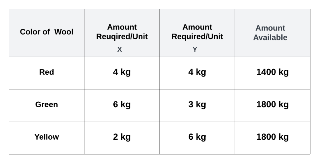
A company makes two types of cloth, X and Y, using three different colors of wool (see Fig 1). Cloth X yields a profit of $12 per unit, while cloth Y yields $8 per unit. The objective is to determine the optimal quantities of X and Y to maximize profit.

Fig. 1

Let $x$ and $y$ denotes the quantities of cloth X and Y produced, respectively. The profit is expressed as

$P = 12x+8y.$

Given that there is only $1400$ kg of red wool available, and each cloth require $4$ kg of red wool, the constraint is

$4x + 4y \le 1400.$

Similarly, considering the available green and yellow wool, the constraints are

$6x + 3y \le 1800, \quad 2x+6y \le 1800.$

Additionally, neither $x$ nor $y$ should be negative,

$x\ge 0, y \ge 0.$

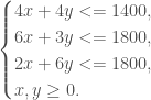
Therefore, the optimization problem can be formulated as:

Maximize the linear objective function

$P=12x+8y$

subject to the linear constraints:

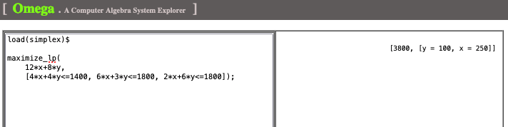
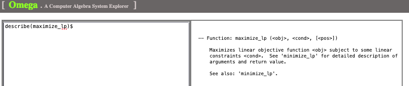
$\begin{cases} 4x+4y<=1400, \\ 6x+3y<=1800, \\ 2x+6y<=1800, \\ x, y \ge 0.\end{cases}$

The problem can be solved using Maxima’s ‘maximize_lp’ :

Fig. 2

The solution in Fig. 3 shows that the company should produce $750$ units of cloth X and $100$ units of cloth Y to achieve the maximum possible profit of $ $3800.$ This will utilize all the available red and green wool, leaving $700$ kg of yellow unused.

Fig. 3

See also “Building the Optimal Portfolio“