An Epilogue of “Analyze This!”

June 29, 2020October 6, 2022 / Michael Xue / Leave a comment

In “Analyze This!“, we examined system

$\begin{cases}\frac{dx}{dt}=n k_2 y - n k_1 x^n \\ \frac{dy}{dt}=k_1 x^n-k_2 y\\x(0)=x_0, y(0)=y_0\;\end{cases}$

qualitatively.

Now, let us seek its equilibrium $(x_*, y_*)$ quantitatively.

In theory, one may first solve differential equation

$\frac{dx}{dt} = -nk_1x^n-k_2x+c_0$

for $x(t)$ , using a popular symbolic differential equation solver such as ‘ode2’. Then compute $x_*$ as $\lim\limits_{t \rightarrow \infty} x(t)$ , followed by $y_* = \frac{k_1}{k_2}x_*^n$ .

However,in practice, such attempt meets a deadend rather quickly (see Fig. 1).

Fig. 1

Bring in a more sophisticated solver is to no avail (see Fig. 2)

Fig. 2

An alternative is getting $x_*$ directly from polynormial equation

$-nk_1x^n-k_2x+c_0=0\quad\quad\quad(1)$

We can solve (1) for $x$ if $n \le 4$ . For example, when $n=3$ , $-3k_1 x^3-k_2x+c_0=0$ has three roots (see Fig. 3).

Fig. 3

First two roots are complex numbers. By Descartes’ rule of signs, the third root

$\frac{(\sqrt{4k_2^3+81c_0^2k_1}+9c_0\sqrt{k_1})^{\frac{2}{3}}-2^{\frac{2}{3}}k_2}{3 \cdot 2^{\frac{1}{3}}\sqrt{k_1}(\sqrt{4k_2^3+81c_0^2k_1}+9c_0\sqrt{k_1})^{\frac{1}{3}}}$

is the $x_*$ of equilibrium $(x_*, y_*)$ (see Exercise-1).

Exercise-1 Show the third root is real and positive.

Exercise-2 Obtain $x_*$ from $-4k_1x^4-k_2x+c_0=0.$

A Delightful Piece of Mathematics

June 22, 2020July 13, 2020 / Michael Xue / Leave a comment

Prove: $\sqrt[3]{\sqrt{108} +10} - \sqrt[3]{\sqrt{108} - 10} = 2.$

We will proceed as follows:

For all $a, b$ ,

$a^3-b^3=(a-b)(a^2+ab+b^2)=(a-b)(a^2-2ab+b^2+3ab)=(a-b)((a-b)^2+3ab)$ .

That is,

$a^3-b^3 = (a-b)((a-b)^2+3ab).\quad\quad\quad(1)$

When

$a = \sqrt[3]{\sqrt{108}+10}, \quad b=\sqrt[3]{\sqrt{108}-10},$

we have

$a^3 = (\sqrt[3]{\sqrt{108}+10})^3 = \sqrt{108}+10, \quad b^3=(\sqrt[3]{\sqrt{108}-10})^3=\sqrt{108}-10.$

It means

$a^3-b^3= 20.$

We also have

$ab = \sqrt[3]{\sqrt{108}+10}\cdot\sqrt[3]{\sqrt{108}-10}=\sqrt[3]{(\sqrt{108})^2-10^2}=\sqrt[3]{8}=2.$

As a result, (1) becomes

$20 = (a-b)((a-b)^2+3\cdot 2).$

Rewrite it as

$20 = x (x^2+6)$

where $x$ denotes $a-b$ , we see that

$a-b=\sqrt[3]{\sqrt{108}+10}-\sqrt[3]{\sqrt{108}-10}$ is a positive root of $20=x(x^2+6).\quad\quad\quad(\star)$

Clearly,

$2$ is also a positive root of $20=x(x^2+6)\quad\quad\quad(\star\star)$

since $20=2\cdot(2^2+6).$

Moreover (see Exercise 1),

$20=x(x^2+6)$ has only one positive root $\quad\quad\quad(\star\star\star)$

Therefore, it must be true that

$\sqrt[3]{\sqrt{108} +10} - \sqrt[3]{\sqrt{108} - 10} = 2.$

Exercise-1 Prove: $20=x(x^2+6)$ has only one positive root.

Exercise-2 Prove: $\sqrt[3]{8+3\sqrt{21}} + \sqrt[3]{8-3\sqrt{21}} = 1$

Analyze This!

June 19, 2020June 26, 2020 / Michael Xue / 4 Comments

Consider the following chemical reaction

$\underbrace{A + A + ... + A}_{n} \underset{k_2}{\stackrel{k_1}{\rightleftharpoons}} A_n$

where $n$ molecule of $A$ combine reversibly to form $A_n$ and, $k_1, k_2$ are the reaction rates.

If $x, y$ are the concentrations of $A, A_n$ respectively, then according to the Law of Mass Action, the reaction is governed by

$\begin{cases}\frac{dx}{dt}=n k_2 y - n k_1 x^n \quad\quad(0-1)\\ \frac{dy}{dt}=k_1 x^n-k_2 y\quad\quad\quad(0-2)\\x(0)=x_0, y(0)=y_0\;\quad(0-3)\end{cases}$

Without solving this initial-value problem quantitatively, the future state of system can be predicted through qualitatively analyzing how the value of $(x, y)$ changes over the course of time.

To this end, we solve (0-1) for $y$ first:

$y=\frac{1}{n k_2}(\frac{dx}{dt} +n k_1 x^n).$

Substitute it in (0-2),

$\frac{d}{dt} (\frac{1}{n k_2}(\frac{dx}{dt} +n k_1 x^n)) =k_1 x^n -k_2 \cdot \frac{1}{n k_2}(\frac{dx}{dt} +n k_1 x^n).$

It simplifies to

$\frac{d^2x}{dt^2} + (n^2 k_1 x^{n-1} + k_2)\frac{dx}{dt} =0.$

Let

$p=\frac{dx}{dt},$

we have

$\frac{d^2x}{dt^2}=\frac{d}{dt}(\frac{dx}{dt})=\frac{dp}{dt}=\frac{dp}{dx}\frac{dx}{dt}=\frac{dx}{dt}\frac{dp}{dx}=p\cdot\frac{dp}{dx}.$

Substituting $p, p\frac{dp}{dx}$ for $\frac{dx}{dt}, \frac{d^2x}{dt^2}$ respectively in (1-1) gives

$p\frac{dp}{dx}+(n^2 k_1 x^{n-1}+k_2)p=0.$

It means $p=0$ or

$\frac{dp}{dx}=-n^2k_1x^{n-1}-k_2.$

Integrate it with respect to $x$ ,

$p = \frac{dx}{dt}=-n k_1 x^n - k_2 x +c_0.$

Let

$f(x) = -n k_1 x^n - k_2 x +c_0$ ,

we have

$\frac{df(x)}{dx} = -n^2 k_1 x^{n-1} - k_2 < 0 \implies f(x) = -n k_1 x^{n-1} - k_2 x + c_0$ is a monotonically decreasing function.

In addition, Descartes’ rule of signs reveals that

$f(x)=0$ has exactly one real positive root.

By definition, this root is the $x_*$ in an equilibrium point $(x_*, y_*)$ .

Fig. 1

Hence,

As time advances, $x\uparrow$ if $x_0 < x_*$ . Otherwise $(x_0>x_*)$ , $x\downarrow \quad\quad\quad(1-1)$

Dividing (0-2) by (0-1) yields

$\frac{dy}{dx} = -\frac{1}{n}.$

That is,

$y=-\frac{1}{n} x + c_1.$

By (0-3),

$c_1 = y_0 + \frac{1}{n}x_0$ .

And so,

$y=-\frac{1}{n} x + y_0 + \frac{1}{n}x_0.$

Since $y$ is a line with a negative slope,

$y$ is a monotonically decreasing function of $x.\quad\quad\quad(1-2)$

Moreover, from (0-1) and (0-2), we see that

$\forall x > 0, (x, \frac{k_1}{k_2}x^n)$ is an equilibrium point.

i.e.,

All points on the curve $y = \frac{k_1}{k_2}x^n$ in the first quadrant of x-y plane are equilibriums $\quad\quad\quad(1-3)$ .

Based on (1-1), (1-2) and (1-3), for a initial state $(x_0, y_0)$ ,

$x_0 < x_* \implies x\uparrow, y\downarrow$ .

Similary,

$x_0 > x_* \implies x\downarrow, y\uparrow$ .

Fig. 2

A phase portrait of the system is shown in Fig. 3.

Fig. 3

It shows that $(x, y)$ on the trajectory approaches the equilibrium point $(x_*, y_*)$ over the course of time. Namely, the system is asymptotically stable.

An Epilogue of “Qualitative Analysis of a Simple Chemical Reaction”

June 8, 2020October 6, 2022 / Michael Xue / Leave a comment

In “Qualitative Analysis of a Simple Chemical Reaction“, we deduced from

$\begin{cases}\frac{dx}{dt}=2 k_2 y - 2 k_1 x^2 \quad\quad(0-1)\\ \frac{dy}{dt}=k_1 x^2-k_2 y\quad\quad\quad(0-2)\end{cases}$

a 1st order differential equation

$\frac{dx}{dt}=-2k_1x^2-k_2x+c_0.$

This differential equation can be solved to obtain $x$ first, then by (0-1),

$y = \frac{1}{2k_2}(\frac{dx}{dt}+2k_1x^2).$

As expected,

$\lim\limits_{t\rightarrow \infty} x(t) = \frac{\sqrt{k_2^2+8c_0k_1}-k_2}{4k_1}=x_*$

and

$\lim\limits_{t\rightarrow \infty} y(t) = -\frac{k_2\sqrt{k_2^2+8c0k_1}-k_2^2-4c_0k_1}{8k_1k_2}=\frac{k_1}{k_2}x_*^2=y_*.$

Exercise-1 Solve differential equation $\frac{dx}{dt}=-2k_1x^2-k_2x+c_0$ without CAS.

Hint: rewrite $\frac{dx}{dt}=-2k_1x^2-k_2x+c_0$ as $\frac{1}{2k_1x^2+k_2x-c_0}\cdot\frac{dx}{dt}=-1.$

Qualitative Analysis of a Simple Chemical Reaction

June 2, 2020June 18, 2020 / Michael Xue / 2 Comments

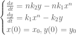
We will study a simple chemical reaction described by

$A + A \underset{k_2}{\stackrel{k_1}{\rightleftharpoons}} A_2$

where two molecules of $A$ are combined reversibly to form $A_2$ and, $k_1, k_2$ are the reaction rates.

If $x$ is the concentration of $A$ , $y$ of $A_2$ , then according to the Law of Mass Action,

$\begin{cases}\frac{1}{2}\cdot\frac{dx}{dt}=k_2 y -k_1 x^2 \\ \frac{dy}{dt}=k_1 x^2-k_2 y\\x(0)=x_0, y(0)=y_0\end{cases}$

or equivalently,

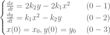
$\begin{cases}\frac{dx}{dt}=2 k_2 y - 2 k_1 x^2 \quad\quad(0-1)\\ \frac{dy}{dt}=k_1 x^2-k_2 y\quad\quad\quad(0-2)\\x(0)=x_0, y(0)=y_0\;\quad(0-3)\end{cases}$

We seek first the equilibrium points that represent the steady state of the system. They are the constant solutions where $\frac{dx}{dt}=0$ and $\frac{dy}{dt}=0$ , simultaneously.

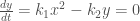From $\frac{dx}{dt}=2 k_2 y - 2 k_1 x^2=0$ and $\frac{dy}{dt}=k_1 x^2-k_2 y=0$ , it is apparent that

$\forall x \ge 0, (x_*, y_*) = (x, \frac{k_1}{k_2}x^2)\quad\quad\quad(0-4)$

is an equilibrium point.

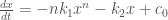
To find the value of $x_*$ , we solve for $y$ from (0-1),

$y = \frac{1}{2k_2}(\frac{dx}{dt}+2 k_1x^2).\quad\quad\quad(0-5)$

Substitute it in (0-2),

$\frac{d}{dt}(\frac{1}{2k_2}(\frac{dx}{dt}+2k_1x^2))=k_1x^2-k_2\frac{1}{2k_2}(\frac{dx}{dt}+2k_1x^2)$

$\implies \frac{d}{dt}(\frac{dx}{dt}+2k_1x^2)=2k_2k_1x^2-k_2(\frac{dx}{dt}+2k_1x^2)$ ,

i.e.,

$\frac{d^2x}{dt^2} + \frac{dx}{dt}(4k_1x+k_2)=0.\quad\quad\quad(0-6)$

This is a 2nd order nonlinear differential equaion. Since it has no direct dependence on $t$ , we can reduce its order by appropriate substitution of its first order derivative.

Let

$p=\frac{dx}{dt}$ ,

we have

$\frac{d^2x}{dt^2} = \frac{d}{dt}(\frac{dx}{dt})=\frac{dp}{dt}=\frac{dp}{dx}\frac{dx}{dt}=\frac{dx}{dt}\frac{dp}{dx}=p\cdot\frac{dp}{dx}$

so that (0-6) is reduced to

$p\cdot\frac{dp}{dx}+p\cdot(4k_1x+k_2)=0,\quad\quad\quad(0-7)$

a 1st order differential eqution. It follows that either $p=\frac{dx}{dt}=0$ or $\frac{dp}{dx}+(4k_1x+k_2)=0$ .

The second case gives

$\frac{dp}{dx}=-4k_1x-k_2.$

Integrate it with respect to $x$ ,

$p=\frac{dx}{dt}=-2k_1x^2-k_2x + c_0.\quad\quad\quad(0-8)$

Hence, the equilibrium points of (0-1) and (0-2) can be obtained by solving a quadratic equation

$-2k_1x^2-k_2x + c_0=0.$

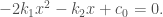
Notice in order to have $x_* \ge 0$ as a solution, $c_0$ must be non-negative .

Fig. 1

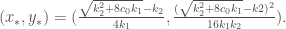
The valid solution is

$x_* = \frac{\sqrt{k_2^2+8c_0k_1}-k_2}{4k_1}.$

Fig. 2

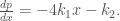
By (0-4),

$y_* =\frac{k_1}{k_2}x_*^2=\frac{(\sqrt{k_2^2+8c_0k_1}-k2)^2}{16k_1 k_2}.$

and so, the equilibrium point is

$(x_*, y_*) = (\frac{\sqrt{k_2^2+8c_0k_1}-k_2}{4k_1}, \frac{(\sqrt{k_2^2+8c_0k_1}-k2)^2}{16k_1 k_2}).$

Next, we turn our attentions to the phase-plan trajectories that describe the paths traced out by the $(x, y)$ pairs over the course of time, depending on the initial values.

For $(x, y) \ne (x_*, y_*), \frac{dx}{dt} \ne 0$ . Dividing (0-2) by (0-1) yields

$\frac{\frac{dy}{dt}}{\frac{dx}{dt}}= \frac{k_1 x^2-k_2 y}{2 k_2 y- 2 k_1 x^2}=-\frac{1}{2}$

i.e.,

$\frac{dy}{dx} = -\frac{1}{2}.$

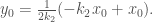
Integrating it with respect to $x$ ,

$y = -\frac{1}{2} x + c_1.$

By (0-3),

$c_1= y_0 +\frac{1}{2}x_0.$

Therefore,

$y = -\frac{1}{2}x +y_0 + \frac{1}{2}x_0.\quad\quad\quad(1-1)$

Moreover, by (0-5)

$y=\frac{1}{2k_2}(\frac{dx}{dt} + 2 k_1 x^2) \overset{(0-8)}{=} \frac{1}{2k_1}(-2k_1 x^2-k_2 x + x_0 +2 k_1 x^2)=\frac{1}{2k_2}(-k_2x +x_0).$

As a result,

$y_0 = \frac{1}{2k_2}(-k_2 x_0 + x_0).$

Substitute $y_0$ in (1-1), we have

$y = -\frac{1}{2} x + \frac{1}{2k_2}(-k_2x_0+x_0) + \frac{1}{2}x_0.$

This is the trajectory of the system. Clearly, all trajectories are monotonically decreaseing lines.

At last, let us examine how the system behaves in the long run.

If $x < x_*$ then $\frac{dx}{dt}>0$ (see Fig. 2) and $x$ will increase. As a result, $y$ will decrease. Similarly, if $x > x_*, \frac{dx}{dt}<0$ ensures that $x$ will decrease. Consequently, $y$ will increase.