On Viete Theorem and Second-Order Linear Differential Equations with Constant Coefficients

December 20, 2017December 12, 2020 / Michael Xue / Leave a comment

Viete theorem, named after French mathematician Franciscus Viete relates the coefficients of a polynomial equation to sums and products of its roots. It states:

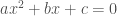
For quadratic equation $a x^2+b x + c =0$ , with roots $r_1, r_2$ ,

$r_1+r_2 = {{-b} \over {a}}$ ,

$r_1 r_2 = {{c} \over {a}}$ .

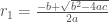
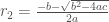
This is easy to prove. We know that the roots of $a x^2 + b x +c =0$ are

$r_1 = {{-b + \sqrt{b^2-4 a c}} \over {2 a}}$ , $r_2 = {{-b - \sqrt{b^2-4 a c}} \over {2 a}}$ .

Therefore,

$r_1 + r_2 ={{-b + \sqrt{b^2-4 a c}} \over {2 a}} + {{-b - \sqrt{b^2-4 a c}} \over {2 a}}={{-b}\over{a}}$

and

$r_1 r_2 = ({{-b + \sqrt{b^2-4 a c}} \over {2 a}})({{-b - \sqrt{b^2-4 a c}} \over {2 a}})={{(-b)^2-(b^2-4 a c)}\over{4 a}}={{c}\over {a}}$ .

In fact, the converse is also true. If two given numbers $r_1, r_2$ are such that

$r_1 + r_2 = {{-b}\over{a}}\qquad\qquad(1)$

$r_1 r_2 = {{c}\over {a}}\qquad\qquad\qquad(2)$

then

$r_1, r_2$ are the roots of $a x^2 + b x + c=0$ .

This is also easy to prove. From (2) we have $r_1 = {{-b}\over{a}}-r_2$ . Hence, (2) implies that $({{-b} \over{a}} -r_2) r_2 = {{c} \over a}$ , or

$a r_2^2 + b r_2 +c =0\qquad\qquad(3)$

Since $r_1, r_2$ are symmetric in both (1) and (2), (3) implies that $r_1$ is also the root of $a x^2 + b x +c = 0$ .

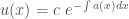
Let us consider the second-order linear ordinary differential equation with constant coefficients:

$y''(t)+b y'(t) + c y = f(t)\qquad\qquad(4)$

Let $\lambda_1, \lambda_2$ be the roots of quadratic equation $x^2+b x + c =0$ with unknown $x$ .

By Viete’s theorem,

$b = -(\lambda_1 + \lambda_2)$

$c =\lambda_1 \lambda_2$ .

Therefore, (4) can be written as

$y''(t)-(\lambda_1+\lambda_2)y'(t) +\lambda_1 \lambda_2 y(t) = f(t)$ .

Rearrange the terms, we have

$y''(t)-\lambda_1 y'(t) - \lambda_2 y'(t) + \lambda_1 \lambda_2 y(t) = f(t)$

i.e.,

$y''(t)-\lambda_1 y'(t) -\lambda_2 (y'(t)-\lambda_1 y(t) )=f(t)$

or,

$(y'(t)-\lambda_1 y(t))' - \lambda_2 (y'(t)-\lambda_1 y(t)) =f(t)\qquad(5)$

Let

$z(t) = y'(t) - \lambda_1 y(t)\qquad\qquad(6)$

(5), a second-order equation is reduced to a first-order equation

$z'(t) - \lambda_2 z(t) = f(t)\qquad\qquad(7)$

To obtain $y(t)$ , we solve two first-order equations, (7) for $z(t)$ first, then (6) for $y(t)$ .

We are now ready to show that any solution obtained as described above is also a solution of (1):

Let $y_*(t)$ be the result of solving (7) for $z(t)$ then (6) for $y(t)$ ,

then

$z(t) = y'_*(t)-\lambda_1 y_*(t)$ .

By (7),

$(y'_*(t)-\lambda_1 y_*(t) )'- \lambda_2(y_*(t)-\lambda_1 y_*(t)) = f(t)\quad\quad\quad(8)$

(8) tells that $y_*(t)$ is a solution of (5).

The fact that (5) is equivalent to (4) implies $y_*(t)$ , a solution of (5) is also a solution of (4)

Solving y’ + a(x) y = b(x), Part 3

December 3, 2017April 29, 2022 / Michael Xue / Leave a comment

Yet another way to find the solution of

$y' + a(x) y = b(x)\quad\quad\quad(1)$

is to seek a function $f(x) > 0 \; \forall x$ such that the result of multiply (1) by $f(x)$ , namely

$f(x)y' + f(x) a(x) y =f(x) b(x)\quad\quad\quad(2)$

can be written as

$(f(x) y)'=b(x) f(x)$ ,

i.e.,

$f(x) y =\int b(x) f(x)\; dx + c_{3}$

where $c_{3}$ is a constant.

Or,

$y = {1 \over f(x)} (\int b(x) f(x)\; dx + c_{3})\quad\quad\quad(3)$

since $f(x) > 0$ .

Let us proceed to find such $f(x)$ .

From (2) we see that if

$f'(x)=a(x) f(x)$

then the left side of (2) is certainly $(f(x) y)'$ and consequently for $f(x) > 0 \;\forall x$ ,

${1 \over f(x)} f'(x) = a(x)\quad\quad\quad(4)$

or,

$log(f(x)) = \int a(x) dx + c_{1}$

where $c_{1}$ is a constant.

Therefore, a solution to (4) is

$f(x) = c_{2}e^{\int a(x)\;dx}\quad\quad\quad(5)$

where $c_{2} = exp(c_{1})$ . This is a positive function $\forall x$ indeed.

With (5), (3) becomes

$y = e^{-\int a(x)\;dx} (\int b(x) e^{ \int b(x) dx} dx + c)\quad\quad\quad(6)$

where $c = {c_{3} \over c_{2}}$ .

In fact, for any constant c,

$e^{-\int a(x) dx} (\int b(x) e^{\int a(x) dx} dx + c)$

is a solution of (1):

$(e^{-\int a(x) dx} (\int b(x) e^{\int a(x) dx} dx+ c))' +$

$a(x)\dot(e^{-\int a(x)\;dx} (\int b(x) e^{\int a(x) dx} dx + c))$

$= -a(x) (e^{-\int a(x) dx} (\int b(x) e^{\int a(x) dx} dx + c))$

$+ e^{-\int a(x) dx} b(x) e^{\int a(x) dx}$

$+ a(x)(e^{-\int a(x) dx} (\int b(x) e^{\int a(x) dx} dx + c))$

$=b(x)$

Therefore, the solution of (1) is

$y = e^{-\int a(x) dx} (\int b(x) e^{\int a(x) dx} dx + c)$

where $c$ is any constant.

Exercise: prove that $e^x$ is a positive function.

Solving y’ + a(x) y = b(x), Part 2

December 2, 2017October 6, 2022 / Michael Xue

In my previous post “Solving y’ + a(x) y = b(x), Part 1“, it was revealed that every solution of

$y' + a(x) y = b(x)\quad\quad\quad(1)$

is the sum of a particular solution, $e^{-\int a(x) dx}\int b(x) e^{\int a(x) dx}dx$ , with $c e^{-\int a(x) dx}$ , a solution of the homogeneous equation $y '+ a(x) y =0$ .

This structure suggests that (1) can be solved in two steps: solve $y' +a(x) y= 0$ first to get $c e^{-\int a(x) dx}$ , then change the constant $c$ in it to a function $c(x)$ and solve for $c(x)$ after submitting the variation into (1).

There is an alternative:

Let

$y = u v$

We have

$(u v)' + a(x) (u v) = v u' + u (v' + a(x) v)=b(x)$

From $v' + a(x) v = 0$ , we obtain

$v = c_1 e^{-\int a(x) dx}$ .

Solving

$v u' = c_1 e^{-\int a(x) dx} u'= b(x)$

subsequently for $u$ yields

$u = \int b(x) e^{\int a(x) dx} dx + c$ .

Hence,

$y = u v = e^{-\int a(x)dx} (\int b(x) e^{\int a(x) dx} dx + c)$ .

Solving y’ + a(x) y = b(x), Part 1

December 2, 2017August 3, 2018 / Michael Xue / 2 Comments

Given a linear differential equation

$y' + a(x) y = b(x)\quad\quad\quad(1)$

It is clear that it has solution $y(x) \equiv 0$ only if $b(x) \equiv 0$ . For if $b(x) \not \equiv 0$ , substituting $y(x) \equiv 0$ into (1) results $0 = b(x), \forall x$ , i.e., $b(x) \equiv 0$ , a contradiction. Hence, when $b(x) \not \equiv 0$ , solution to (1) must be a function $y(x) \not \equiv 0$ . If the solution is not everywhere zero, then for $y(x) \neq 0$ , we have

$y' = ({b(x) \over y} -a(x)) y$

or equivalently

${1 \over y} y' = {b(x) \over y} -a(x)$ ,

from which we conclude

$log(|y|) = \int {{b(x) \over y} - a(x)} dx + c_1$

where $c_1$ is a constant.

It follows that

$y = c_2 e^{\int {{b(x) \over y} - a(x)} dx}\quad\quad\quad(2)$

where $c_2$ is either $+e^{c_1}$ if $y >0$ or $-e^{c_1}$ if $y < 0$ .

We can express (2) differently as

$y = c_2 e^{\int {b(x) \over y} dx} e^{- \int a(x) dx}\quad\quad\quad(3)$ ,

where $c_2 e^{\int { b(x) \over y} dx}$ is clearly a function of $x$ .

Let

$y = \phi(x) e^{-\int a(x) dx}\quad\quad\quad(4)$

we have

$(\phi(x) e^{-\int a(x) dx})' + a(x) \phi(x) e^{-\int a(x) dx}$

$= \phi'(x)e^{-{\int a(x) dx}}-\phi(x) a(x) e^{-\int a(x) dx} + a(x) \phi(x) e^{-\int a(x) dx}$

$= \phi'(x) e^{-\int a(x) dx}=b(x)$ .

Hence,

$\phi(x) = \int {b(x) e^{\int a(x) dx} dx} + c\quad\quad\quad(5)$

where $c$ is a constant.

With (5), (4) becomes

$y = e^{-\int a(x) dx} (\int{b(x) e^{\int a(x) dx}} dx + c)\quad\quad\quad(6)$

As a matter of fact, for any constant $c$ , (6) is a solution of (1):

$(e^{-\int a(x) dx} (\int{b(x) e^{\int a(x) dx}} dx + c)' + a(x) e^{-\int a(x) dx} (\int{b(x) e^{\int a(x) dx}} dx + c)$

$=-a(x) e^{-\int a(x) dx}(\int {b(x) e^{\int a(x) dx}} dx + c)+e^{-\int a(x) dx}b(x)e^{\int a(x) dx}$

$+ a(x) e^{-\int a(x) dx} (\int b(x)e^{\int a(x) dx} +c)$

$= b(x)$

Notice when $b(x)=0, c=0$ , (6) yields $y(x) \equiv 0$ .

Consequently, (6) defines a family of (1)’s solution.

But are there any other solutions ?

To answer this question, let us first rewrite (6) as

$y = e^{-\int a(x) dx} \int{b(x) e^{\int a(x) dx}} dx + ce^{-\int a(x) dx}\quad\quad\quad(7)$

We see that $e^{-\int a(x)dx}\int{b(x) e^{\int a(x) dx} }dx$ is a solution of (1) since it is the $y(x)$ of (7) when $c =0$ .

Let $y(x)$ denotes any solution of (1) and,

$y_*(x) = e^{-\int a(x) dx} \int{b(x) e^{\int a(x) dx}} dx$ ,

$z(x) = y(x) - y_*(x)$

Since $y'(x)+a(x)y=b(x), y_*'(x)+a(x)y_*(x)=b(x)$ ,

$z'(t) + a(x) z(t)$

$= (y(x)-y_*(x))' + a(x)(y(x)-y_*(x))$

$= y'(x)-y_*'(x)+a(x)y(x)-a(x)y_*(x)$

$= y'(x) + a(x)y(x) - (y_*'(x)+a(x) y_*(x))$

$= b(x) - b(x)$

$= 0$ .

It means $z(x)$ is a solution of $y'+a(x)y=0$ .

We know $c e^{-\int a(x) dx}$ is the solution of $y'+a(x) y=0$ (see “Solving y’+a(x) y =0“)

Therefore,

$y(x) - y_*(x) = c e^{-\int a(x) dx}$ ,

i.e.,

$y(x) = y_*(x) + c e^{-\int a(x) dx}$

or,

$y(x) = e^{-\int a(x) dx}( \int{b(x) e^{\int a(x) dx}} dx + c)$ .

Thus, we have shown that all solutions of (1) are of the form (6)!

Stated differently,

The collection of functions expressed by

$y = e^{-\int a(x) dx} (\int{b(x) e^{\int a(x) dx}} dx + c)$

where $c$ is any constant constitutes all possible solutions of $y' + a(x) y =b(x)$ .

Solving y’ + a(x) y = 0

December 1, 2017August 3, 2018 / Michael Xue / 2 Comments

Let’s consider the 1st-Order linear differential equation

$y'(x)+ a(x) y(x) =0\quad\quad\quad(1)$

We see $y(x) \equiv 0$ is a solution.

However, if (1) has a solution whose value at $x$ is not zero, it must be true that

${1 \over y(x)} y(x)' = -a(x)$

i.e.,

$log(|y(x)|) = -\int a(x) dx + c_1\quad\quad\quad(2)$

where $c_1$ is a constant.

From (2), we obtain

$y(x) = c\;e^{-\int a(x) dx}\quad\quad\quad(3)$

where $c$ is a constant. It is either $+e^{c_1}$ or $-e^{c_1}$ .

We assert and prove that for any constant $c$ , a function defined by (3) is a solution of (1):

$(c\;e^{-\int a(x)dx)})' +a(x)c\;e^{-\int a(x) dx}=-c\;a(x)e^{-\int a(x) dx} +a(x) c\;e^{-\int a(x) dx} =0$ .

Notice when $c=0$ , (3) yields $y(x) \equiv 0$ , the zero solution of (1).

Moreover, to see there are no other solutions, let $u(x)$ be any solution of (1), we have

$(u(x) e^{\int a(x)dx})' = u'(x) e^{\int a(x) dx} + u(x) a(x) e^{\int a(x) dx}$

$= e^{\int a(x)dx } (u'(x) + a(x) u(x))$

$= 0$ .

Therefore,

$(u(x) e^{\int a(x) dx})' = 0$ .

That is

$u(x) e^{\int a(x)dx} = c$

or,

$u(x) = c\;e^{-\int a(x) dx}$

where $c$ is a constant. Hence, any solution of (1) belongs to the family of functions defined by (3)