The above animation is produced by Omega CAS Explorer:


Research on rocket flight performance has shown that typical single-stage rockets cannot serve as the carrier vehicle for launching satellite into orbit. Instead, multi-stage rockets are used in practice with two-stage rockets being the most common. The jettisoning of stages allows decreasing the mass of the remaining rocket in order for it to accelerate rapidly till reaching its desired velocity and height.
Optimizing flight performance is a non-trivial problem in the field of rocketry. This post examines a two-stage rocket flight performance through rigorous mathematical analysis. A Computer Algebra System (CAS) is employed to carry out the symbolic computations in the process. CAS has been proven to be an efficient tool in carry out laborious mathematical calculations for decades. This post reports on the process and the results of using Omega CAS explorer, a Maxima based CAS to solve this complex problem.
A two-stage rocket consists of a payload 


Based on Tsiolkovsky’s equation, we derived the multi-stage rocket flight equation ![[1]](https://s0.wp.com/latex.php?latex=%5B1%5D&bg=ffffff&fg=444444&s=0&c=20201002)
Let 
where 
We seek an appropriate value of 

Consider 

Fig. 1
We have 
That is, 

Fig. 2
As shown in Fig. 2,
Notice that 
Solving 


Fig. 3
We rewrite the expression under the square root in 


Fig. 4
If 


The expression under the square root is positive means both 


Fig. 5
From (3) where 
For all 

For all 
For all 

Fig. 6
Moreover, from Fig. 6,

Since the expression in the numerator of 

It follows that
The implication is that 

However, if both 


We will proceed to show that the only zero lies between
There are two cases to consider.
Case 1 (


Case 2 (


The fact that only 

Fig. 7
The result 


To obtain a correct Taylor series expansion for 
Its first order Taylor series is then computed (see Fig. 8)

Fig. 8
The first term of the result can be written as 

To compute 


Fig. 9
Writing its first term as
It is positive when
We have shown the time-saving, error-reduction advantages of using CAS to aid manipulation of complex mathematical expressions. On the other hand, we also caution that just as is the cases with any software system, CAS may contain software bugs that need to be detected and weeded out with a well- trained mathematical mind.
References
![[2]](https://s0.wp.com/latex.php?latex=%5B2%5D&bg=ffffff&fg=444444&s=0&c=20201002)

There is another way to obtain the results stated in “Finite Difference Approximations of Derivatives“.
Let 


We define

By Taylor’s expansion around 
Substituting (1-1), (1-2) into (1),

That is,
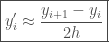
It follows that

Fig. 1
Solving (1-3) for 
Therefore,
or,
Now, let

From
and
we have,

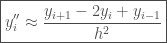
It leads to

Fig. 2
whose solution (see Fig. 2) is

Hence,
i.e.,