A Gift That Keeps On Giving

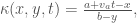
We see from “Seek-Lock-Strike!” Again that given the missile’s position (x, y),

\frac{dx}{dy}=\frac{a+v_a t-x}{b-y}

where x and y are themselves functions of time t.

It means

\frac{dx}{dy} = \frac{\frac{dx}{dt}}{\frac{dy}{dt}}=\frac{a+v_a t-x}{b-y}\implies \frac{dx}{dt} = \frac{a+v_a t-x}{b-y}\cdot\frac{dy}{dt}.

That is, let \kappa(x,y,t) = \frac{a+v_a t-x}{b-y},

\frac{dx}{dt}=\kappa\cdot \frac{dy}{dt}.\quad\quad\quad(1)

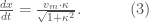
We also have (see “Seek-Lock-Strike!”)

v_m = \sqrt{(\frac{dx}{dt})^2+(\frac{dy}{dt})^2}\implies v_m = \sqrt{1+\kappa^2}|\frac{dy}{dt}| .

Since \frac{dy}{dt} >0,

\frac{dy}{dt} = \frac{v_m}{\sqrt{1+\kappa^2}}.\quad\quad\quad(2)

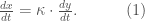
Substitute (2) into (1) yields

\frac{dx}{dt} = \frac{v_m\cdot \kappa}{\sqrt{1+\kappa^2}}.\quad\quad\quad(3)

It follows that (x(t), y(t)), the position of the missile satisfies the initial-value problem

\begin{cases} \frac{dx}{dt} = \frac{\kappa\cdot v_m}{\sqrt{1+\kappa^2}} \\ \frac{dy}{dt} = \frac{v_m}{\sqrt{1+\kappa^2}} \\x(0)=0, y(0)=0\end{cases}\quad\quad\quad(4)

To obtain the missile’s trajectory, we solve (4) numerically using the Runge-Kutta algorithm. It integrates (4) from t=0 to t= t_* (see “Seek-Lock-Strike!”).

Fig. 1 a=100\;m, b=3000\;m, v_a=1500\;ms^{-1},v_m=2000\;ms^{-1}

The missile strike is illustrated in Fig. 1 and 2.

Fig. 2 a=100\;m, b=3000\;m, v_a=1500\;ms^{-1},v_m=2000\;ms^{-1}

Fig. 3 a=-1200\;m, b=3000\;m, v_a=1500\;ms^{-1},v_m=2000\;ms^{-1}

The trajectories shown are much smoother than those in “Seek-Lock-Strike!” Animated.