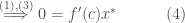
Finding the value of for is equivalent to seeking a positive number whose square yields : . In other words, the solution to .
We can find by solving . It is by mere inspection. can also be obtained by solving , again, by mere inspection. But ‘mere inspection’ can only go so far. For Example, what is ?
Method for finding the square root of a positive real number date back to the acient Greek and Babylonian eras. Heron’s algorithm, also known as the Babylonian method, is an algorithm named after the – century Greek mathematician Hero of Alexandria, It proceeds as follows:
Begin with an arbitrary positive starting value .
Let be the average of and
Repeat step 2 until the desired accuracy is achieved.
This post offers an analysis of Heron’s algorithm. Our aim is a better understanding of the algorithm through mathematics.
Let us begin by arbitrarily choosing a number . If , then is , and we have guessed the exact value of the square root. Otherwise, we are in one of the following cases:
Case 1:
Case 2:
Both cases indicate that lies somewhere between and .
Let us define as the relative error of approximating by :
The closer is to , the better is as an approximation of .
Since ,
By (1),
Let be the mid-point of and :
and, the relative error of approximating ,
We have
By (5),
i.e., lies between and .
We can generate more values in stages by
Clearly,
.
Let
.
We have
and
Consequently, we can prove that
by induction:
When .
Assume when ,
When .
Since (11) implies
(10) and (13) together implies
It follows that
and
(15) indicates that the error is cut at least in half at each stage after the first.
Therefore, we will reach a stage that
It can be shown that
by induction:
When ,
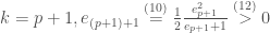
Assume when k = p,
When ,
From (17) and (18), we see that the error decreases quadratically.
Illustrated below is a script that implements the Heron’s Algorithm:
/*
a   - the positive number whose square root we are seeking
x0  - the initial guess
eps - the desired accuracy
*/
square_root(a, x0, eps) := block(
    [xk],
    numer:true,
    xk:x0,
    loop,
        if abs(xk^2-a) < eps then return(xk),
        xk:(xk+a/xk)/2,
    go(loop)
)$
Suppose we want to find and start with . Fig. 2 shows the Heron’s algorithm in action.
The stages of a two stage rocket have initial masses and respectively and carry a payload of mass . Both stages have equal structure factors and equal relative exhaust speeds. If the rocket mass, , is fixed, show that the condition for maximal final speed is
.
Find the optimal ratio when .
According to multi-stage rocket’s flight equation (see “Viva Rocketry! Part 2“), the final speed of a two stage rocket is
Let , we have
and,
Differentiate with respect to gives
It follows that implies
.
That is, . i.e.,
It is the condition for an extreme value of . Specifically, the condition to attain a maximum (see Exercise-2)
When , solving
yields two pairs:
and
Only (3) is valid (see Exercise-1)
Hence
The entire process is captured in Fig. 2.
Fig. 2
Exercise-1 Given , prove:
Exercise-2 From (1), prove the extreme value attained under (2) is a maximum.
The stages of a two-stage rocket have initial masses and respectively and carry a payload of mass . Both stages have equal structure factors and equal relative exhaust speed . The rocket mass, is fixed and .
According to multi-stage rocket’s flight equation (see “Viva Rocketry! Part 2“), the final speed of a two-stage rocket is
Let , it becomes
where . We will maximize with an appropriate choice of .
That is, given
where . Maximize with an appropriate value of .
The above optimization problem is solved using calculus (see “Viva Rocketry! Part 2“). However, there is an alternative that requires only high school mathematics with the help of a Computer Algebra System (CAS). This non-calculus approach places more emphasis on problem solving through mathematical thinking, as all symbolic calculations are carried out by the CAS (e.g., see Fig. 2). It also makes a range of interesting problems readily tackled with minimum mathematical prerequisites.
The fact that
is a monotonic increasing function
where
or
(1) can be written as
where
,
.
Since means
.
That is
.
Solve
for gives if .
Hence, (1) is a quadratic equation. For it to have solution, its discriminant must be nonnegative, i.e.,
Consider
If , (3) is a quadratic equation.
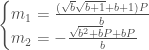
Solving (3) yields two solutions
,
.
Since ,
(4) implies
and, the solution to (2) is
or
i.e.,
or
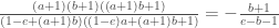
We prove that (4) is true by showing (5) is false:
Consider :
where
.
It can be written as
where
,
,
.
Since (see Exercise 1) and,
solve (7) for yields
.
It follows that for .
Consequently, is a negative quantity. i.e.,
which tells that (5) is false.
Hence, when , the global maximum is .
Solving for :
,
we have
.
Therefore,
attains maximum at .
In fact, attains maxima at even when , as shown below:
Solving for , we have
or .
Only is valid (see Exercise-2),
When ,
where
Solve quadratic equation for yields
.
The coefficient of in is , a negative quantity (see Exercise-3).
The implication is that is a negative quantity when .


 for
for  is equivalent to seeking a positive number
  :
:  . In other words, the solution to
  .
. by solving
  . It is
  by mere inspection.
  can also be obtained by solving
  , again, by mere inspection. But ‘mere inspection’ can only go so far. For Example, what is
  ?
? – century Greek mathematician Hero of Alexandria, It proceeds as follows:
 .
. be the average of
  and
and 
 . If
. If  , then

 and
and  as the relative error of approximating
 ,
,

 be the mid-point of
 the relative error of


 and
and 
 .
. .
.


 .
. ,
, 
 .
.


 that
that

 ,
,

 ,
,
 and start with
  . Fig. 2 shows the Heron’s algorithm in action.

 and
and  respectively and carry a payload of mass
  . Both stages have equal structure factors and equal relative exhaust speeds. If the rocket mass,
  , is fixed, show that the condition for maximal final speed is
  .
. when
when  .
.
 , we have

 with respect to
 implies
 .
. . i.e.,


 , prove:
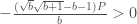


 and equal relative exhaust speed
  . The rocket mass,
  .
.
 , it becomes
 . We will maximize
  with an appropriate choice of
 . Maximize
  is a monotonic increasing function


 ,
, .
. means
means  .
. .
.
 gives
gives  if
if  .
. must be nonnegative, i.e.,

 , (3) is a quadratic equation.
 ,
,  .
. ,
,

 or
or 


 :
:


 .
.

 ,
,
 ,
,
 .
. (see Exercise 1) and,
 .
. .
.  is a negative quantity. i.e.,
 is
is  .
. for
for  ,
, .
. attains maximum at
  attains maxima at
  even when
  , as shown below:
 or
or  .
. ,
,

 for
for  in
in  is
is  , a negative quantity (see Exercise-3).
 .
.
 attains its maximum at


 as a polynomial. Namely,
 .
. , i.e.,
 s are constants.
 ,
, 
 .
. is a polynomial:
 ,
,  .
.


 .
. .
.
 s are constants.
 , (3) becomes

 ,
,
