In this appendix to my previous post “From Dancing Planet to Kepler’s Laws“, we derive the polar form for an ellipse that has a rectangular coordinate system’s origin as one of its foci.
Fig. 1
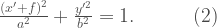
We start with the ellipse shown in Fig. 1. Namely,
Clearly,
After shifting the origin to the right by , the ellipse has the new origin as one of its foci (Fig. 2).
Fig. 2
Since , the ellipse in is
Substituting in (2) by
yields equation
Replacing by respectively, the equation becomes
Fig. 3
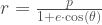
Solving (3) for (see Fig. 3) gives
or .
The first solution
.
Let
,
we have
.
The second solution is not valid since it suggests that :
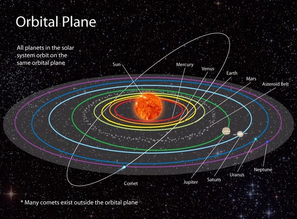
“This most beautiful system of the sun, planets, and comets, could only proceed from the counsel and dominion of an intelligent powerful Being” – Sir. Issac Newton
When I was seven years old, I had the notion that all planets dance around the sun along a wavy orbit (see Fig. 1).
Fig. 1
Many years later, I took on a challenge to show mathematically the orbit of my ‘dancing planet’ . This post is a long overdue report of my journey.
Shown in Fig. 2 is the sun and a planet in a x-y-z coordinate system. The sun is at the origin. The moving planet’s position is being described by .
Fig. 2
According to Newton’s theory, the gravitational force sun exerts on the planet is
where is the gravitational constant, the mass of the sun and planet respectively. .
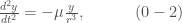
By Newton’s second law of motion,
(0-3) (0-2) yields
.
Since
,
it must be true that
.
i.e.
where is a constant.
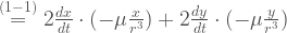
Similarly,
where are constants.
Consequently,
,
,
.
Hence
If then by the following well known theorem in Analytic Geometry:
“If A, B, C and D are constants and A, B, and C are not all zero, then the graph of the equation Ax+By+Cz+D=0 is a plane“,
(0-7) represents a plane in the x-y-z coordinate system.
For , we have
.
It means
where is a constant. Simply put,
.
Hence, (0-7) still represents a plane in the x-y-z coordinate system (see Fig. 3(a)).
Fig. 3
The implication is that the planet moves around the sun on a plane (see Fig. 4).
Fig. 4
By rotating the axes so that the orbit of the planet is on the x-y plane where (see Fig. 3), we simplify the equations (0-1)-(0-3) to
It follows that
.
i.e.,
.
Integrate with respect to ,
where is a constant.
We can also re-write (0-6) as
where is a constant.
Using polar coordinates
Fig. 5
we obtain from (1-2) and (1-3) (see Fig. 5):
If the speed of planet at time is then from Fig. 6,
Fig. 6
gives
Suppose at , the planet is at the greatest distance from the sun with and speed . Then the fact that attains maximum at implies . Therefore, by (1-4) and (1-5),
i.e.,
We can now express (1-4) and (1-5) as:
Let
then
By chain rule,
.
Thus,
.
That is,
Since
,
we let
.
Notice that .
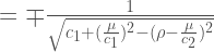
By doing so, (1-14) can be expressed as
.
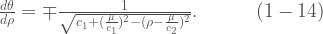
Take the first case,
.
Integrate it with respect to gives
where is a constant.
When ,
or .
And so,
or .
For ,
.
By (1-11), it is
Fig. 7
Solving (1-15) for yields
.
i.e.,
Studies in Analytic Geometry show that for an orbit expressed by (1-16), there are four cases to consider depend on the value of :
We can rule out parabolic and hyperbolic orbit immediately for they are not periodic. Given the fact that a circle is a special case of an ellipse, it is fair to say:
The orbit of a planet is an ellipse with the Sun at one of the two foci.
In fact, this is what Kepler stated as his first law of planetary motion.
Fig. 8
For ,
from which we obtain
This is an ellipse. Namely, the result of rotating (1-16) by hundred eighty degrees or assuming attains its minimum at .
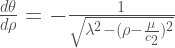
The second case
can be written as
.
Integrate it with respect to yields
from which we can obtain (1-16) and (1-17) again.
Fig. 9
Over the time duration , the area a line joining the sun and a planet sweeps an area (see Fig. 9).
.
It means
or that
is a constant. Therefore,
A line joining the Sun and a planet sweeps out equal areas during equal intervals of time.
This is Kepler’s second law. It suggests that the speed of the planet increases as it nears the sun and decreases as it recedes from the sun (see Fig. 10).
Fig. 10
Furthermore, over the interval , the period of the planet’s revolution around the sun, the line joining the sun and the planet sweeps the enire interior of the planet’s elliptical orbit with semi-major axis and semi-minor axis . Since the area enlosed by such orbit is (see “Evaluate a Definite Integral without FTC“), setting in (2-1) to gives


 .
.


 is the gravitational constant,
  the mass of the sun and planet respectively.
  .
.

 (0-3)
(0-3)  (0-2) yields
 .
. ,
, .
.
 is a constant.

 are constants.
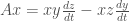 ,
, ,
, .
.

 then by the following well known theorem in Analytic Geometry:
 , we have
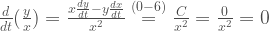 .
.
 is a constant. Simply put,
  .
.

 (see Fig. 3), we simplify the equations (0-1)-(0-3) to


 .
. .
. ,
,
 is a constant.
 is a constant.


 then from Fig. 6,


 , the planet is at the greatest distance from the sun with
  and speed
  . Then the fact that
  . Therefore, by (1-4) and (1-5),


 .
.


 .
.
 ,
, .
. .
. .
. .
. gives
gives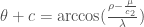
 is a constant.
 or
or  .
. or
or  .
. ,
,  .
.

 .
.
 :
:

 ,
,


 .
.

 , the area a line joining the sun and a planet sweeps an area
  .
.


 , the period of the planet’s revolution around the sun, the line joining the sun and the planet sweeps the enire interior of the planet’s elliptical orbit with semi-major axis
  and semi-minor axis
  . Since the area enlosed by such orbit is
  (see “
 in (1-16), it is also true that for such ellipse,
  (see “
 in (3-1),


 ,
,  .
. .
. is a quarter of the area enclosed by a circle with radius
  .
. .
.